Finding Reliable Communication Backbones in a Wireless Sensor Network

Nearing the end of my master's degree I had the pleasure of taking Algorithms Engineering with Dr. David Matula, who has done a significant amount of work in the graph theory space. For my end of semester project I created a program and corresponding visualization that was targeted at finding communication backbones in wireless sensor networks.

As it turns out random geometric graphs (RGG) are extremely good at modeling wireless sensor networks. This is because an RGG's edges are determined by a vertex's proximity to another vertex. These two vertices have an edge between them if they are less than some distance r from each other. In this case r is an analog to the broadcast radius of a wireless sensor. In a real world wireless sensor network, sensors may be dropped from a plane or scattered on the ground in some unpredictable fashion. It is useful to be able to create a communication backbone between these sensors so that you can extract data from all the sensors from only one (or very few) egress sensors. Imagine that it would be much nicer to walk to and download information from one sensor than to gather information individually from all sensors that are scattered throughout some arbitrarily large geographic area. Using "smallest last ordering" and graph coloring algorithms were able to reliably choose pretty good backbones, using a program and any random geometric graph as input. This project was extremely in depth so I recommend that you click here to explore the project further and read the whole project description as well as check out the cool visualizations I made to display the work that has been done.

This project has to be one of the coolest that I worked on at University. The task was centered around reliably finding high quality communication backbones in a wireless sensor network. This is becoming increasingly relevant as IoT devices are becoming cheaper and more ubiquitous by the day. Consider an example where thousands of wireless sensors are thrown out at random across a planet's surface. It would be very costly and time consuming to travel to each individual sensor and extract its stored information. Instead it would be vastly superior if it were possible to extract information from the entire network from only one single egress point. To do this we need to establish communication backbones that will identify routes for this information to flow out of the network.

To simulate the behavior of such a network, we used random geometric graphs (RGGs). RGGs have the property that a vertex is connected to another vertex if it is within some distance R of each other, where R is a configurable distance and is a very apt analog to broadcast range on a wireless sensor. Then using a pretty massive series of graph algorithms to color, order and select nodes, we generate some viable backbones. To give you an idea of how this works, we first perform a "Smallest Last Ordering" of the nodes in the graph and then color them based on this ordering. This ordering and then subsequent coloring allows us to identify maximum independent sets of nodes with a bias towards high degree nodes. This means that colors generated early (color 0 in terms of the Grundy coloring algorithm) will generally have many many nodes in it with extremely high set coverage. We can then combine any two of these independent sets and pick the ones with the highest overall set coverage (and potentially fewest number of vertices). This is best demonstrated by example. Please watch the following video visualizing the results on a unit sphere.

sphereVisualizationDemo from Tyler Springer on Vimeo.

This project has two major components:

• The Visualization Component
• The Computation Component

Visualization was done entirely using the Processing language by reading in data that was pre-generated by the Computation Component. The visualization component is demoed above, but only results for the sphere is shown. In addition to a sphere, I also tested graphs with points thrown onto a unit square and also a unit disk. Here are some sample images of those in action:

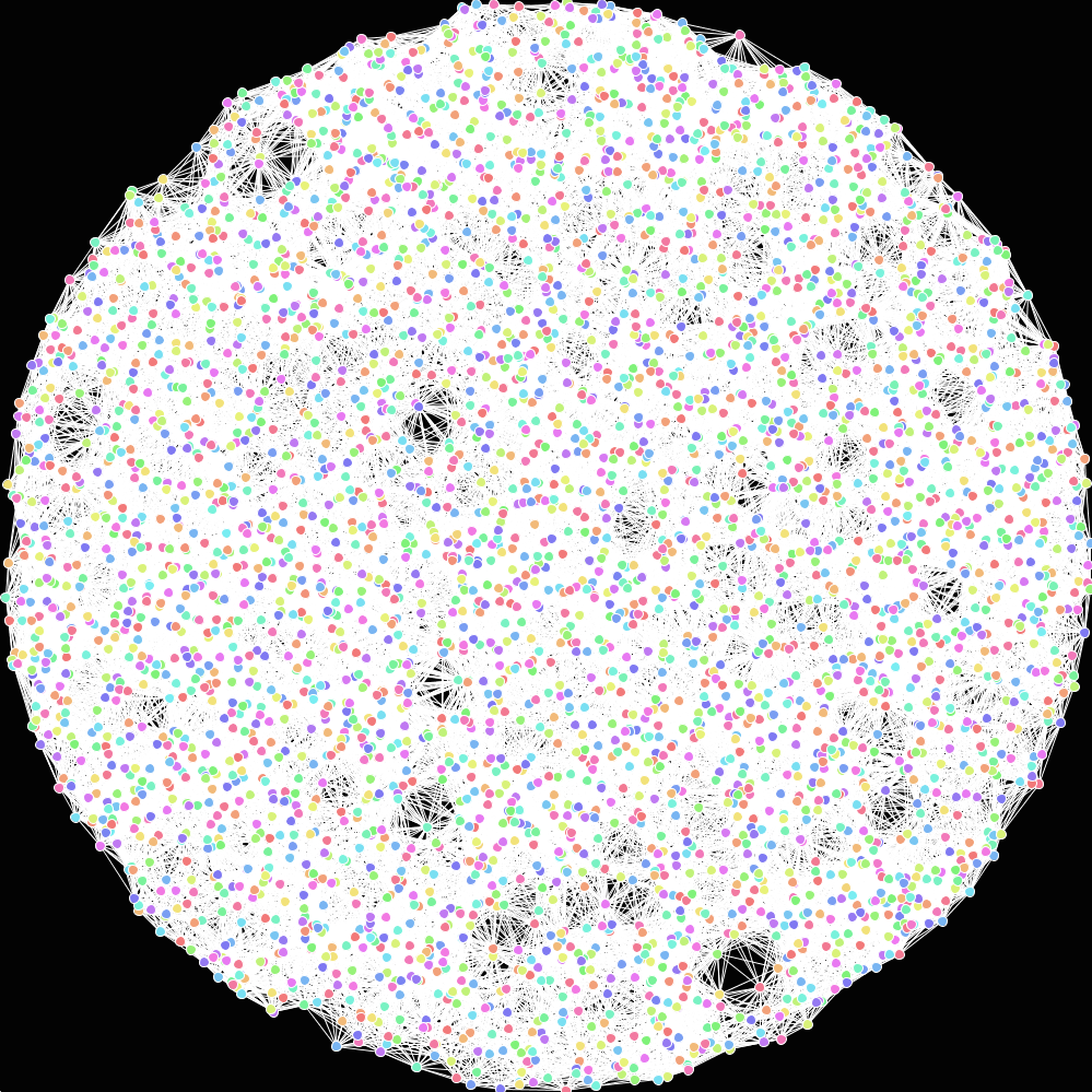
And here is a communication backbone generated for this graph (it has 99.95% set coverage).

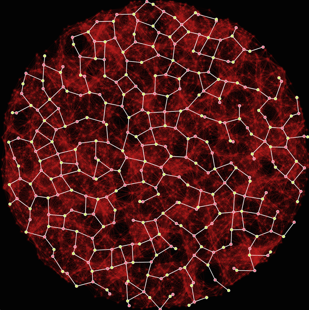
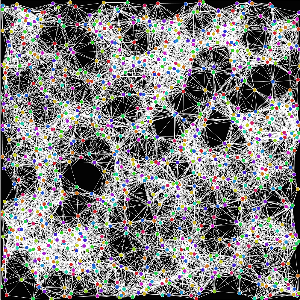
And here's a graph on a unit square just because it looks pretty:

The computation component is responsible for actually creating all this data. Is is a python/C program (using Cython to expedite the process of writing a C extension) that creates a number of CSV files that are then visualized by the Processing sketches shown above. This program is a command line utility that I created to nicely and quickly generate all the required data for a simulation. Input parameters include the number of nodes, the type of projection (square, disk, sphere), the evaluation method, the average degree of nodes within the graph and the location where you'd like the files written to.

One other interesting feature of this program is that there are a number of optimizations to help reduce computational complexity (this really helps when graphs become large). For example, when generating graphs we must compare the distance of each node to every other node in order to determine whether or not they are less than or equal to a distance R from each other and thereby have a connecting edge which given n nodes will take n^2 comparisons to evaluate, or O(n^2). That's not a great running class to be in, so instead it make a lot more sense to optimize this process. Given the observation that nodes that are greater than a distance R from each other cannot be connected, it doesn't make a lot of sense for nodes on opposite sides of the graph to be compared as its physically impossible that they are connected. So instead it is much better if we divide the graph up into a grid where each cell is RxR in size. We then compare the nodes only within that cell to each other eliminating silly comparisons that will objectively never result in an edge between vertices. This process runs in O(n^2 r^2) where R is less than 1. This is only one example of optimizations that makes this a tractable problem and one that can actually be implemented in the real world.

The post below is the actual document I submitted for my project and is chock full of more details about this whole process. Please take a moment to read through it as you might learn something interesting!